Randomized Optimization & Clustering Benchmarks
Two CS7641 studies benchmarking randomized search heuristics on discrete problems and neural network weights, and clustering with dimensionality reduction on stock and tennis datasets.
Project Overview
Two empirical studies from CS7641 Machine Learning at Georgia Tech, Summer 2024. The first benchmarks randomized search heuristics on discrete optimization problems and then turns them loose on neural network weights. The second asks what happens to clustering when the feature space is projected down first. Both are single-author work.
The two studies share a dataset. Stock market data for the JPM symbol from 2009 to 2021 appears in both, and the tennis match dataset from my CSE6242 project is reused as the second clustering dataset.
Part I: Randomized Optimization Heuristics
Gradient methods need a differentiable loss surface. When the surface is discrete or riddled with local optima, randomized search is the alternative. This study compares four heuristics implemented with mlrose-hiive: Randomized Hill Climbing (RHC), Simulated Annealing (SA), Genetic Algorithms (GA), and Mutual-Information-Maximizing Input Clustering (MIMIC). Gradient Descent (GD) is included only as a benchmark on the neural network task.
The problems
Two classic discrete problems were chosen to stress different behaviours:
- Flip Flop (FFP), at string lengths 40, 100, and 500. Fitness counts alternating bit transitions, so the landscape is full of shallow local optima that punish greedy search.
- N-Queens (NQP), at board sizes 20, 50, and 100. A constraint satisfaction problem whose search space grows exponentially and whose row, column, and diagonal constraints must all hold at once.
Algorithms
Simulated Annealing accepts a worsening move with probability
\[P(\text{accept}) = \exp\left(-\frac{\Delta E}{T}\right)\]for $\Delta E > 0$, under a geometric cooling schedule $T_k = T_0 \cdot \alpha^k$. The study swept decay = 0.95 with geometric, arithmetic, and exponential decay variants and initial temperatures from 1 to 10.
MIMIC fits a probability distribution over the top $\theta$-percentile of candidates and builds a dependency tree over the variables:
\[P(X_1, X_2, \dots, X_n) = P(X_{i_1}) \prod_{j=2}^{n} P(X_{i_j} \mid X_{i_{\pi(j)}})\]where $\pi(j)$ is the parent of index $j$ in the tree. It captures variable dependencies that RHC and SA cannot see, at a substantial computational cost.
Results on the discrete problems
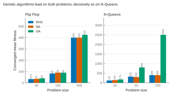
GA converges fastest and highest on both problems. On Flip Flop the three algorithms end up close together, with GA reaching its plateau within roughly 20 to 50 iterations while RHC needs several hundred. On N-Queens the separation is decisive: GA’s population-based crossover handles the simultaneous row, column, and diagonal constraints in a way that single-point search does not, and by board size 100 it reaches a converged fitness several times that of RHC or SA.
RHC converges quickest of all but is the least reliable, showing the highest variability and the strongest sensitivity to its restart strategy. SA sits between the two: volatile early, then steady, with its probabilistic acceptance of worse solutions doing exactly what the cooling schedule is meant to do.
Results on neural network weights
The third task replaced backpropagation with randomized search for the weights of a network predicting buy and sell signals on JPM stock, using 2,159 training and 926 test samples across 18 technical-indicator features. Across 272 runs sweeping hidden layer sizes, activation functions, population sizes, and cooling schedules:
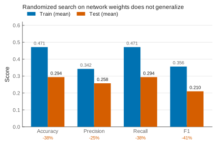
This is a negative result and worth reporting as one. Mean test accuracy is 0.294 against 0.471 on train, and mean test F1 is 0.210 against 0.356. Wall-clock cost varied from 3.6 seconds to nearly 5,000 seconds across configurations.
One caveat has to come before any interpretation of those numbers. On a binary task, chance is 0.5, and both the test mean (0.294) and the train mean (0.471) sit below it, with a test median of 0.227. A classifier performing that far under chance on both splits usually indicates a defect in the evaluation rather than a property of the search algorithms. The report’s accuracy definition is written as $(TP+TN+FP+FN)/(TP+TN)$, which is inverted, and accuracy equals recall at every quantile in Table IV. I am reporting the table as published, but I would not draw an algorithmic conclusion from it without recomputing the metrics.
MIMIC is introduced above as the fourth heuristic but appears in none of the results: the report’s MIMIC subsection is empty and its hyperparameters are listed as not applicable, so only three algorithms are plotted.
The mean also hides how wide the spread is. Table IV reports a full five-number summary over the 272 runs, which is exactly what a box plot encodes:
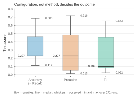
The best single configuration reached a test F1 of 0.653, close to the tennis classifier’s 0.733 on a different problem. But the median run scored 0.102. On this task the choice of hidden layers, activation, population size and cooling schedule matters more than the choice of search algorithm.
The report concludes that gradient descent remains the better choice for this task on both efficiency and generalization, with SA and GA justified only where the loss surface is genuinely non-smooth. Given the metric problem above, that conclusion is not supported by this table, whatever its merits on other grounds.
Part II: Clustering & Dimensionality Reduction
The second study pairs two clustering algorithms with three dimensionality reduction techniques and measures what the projection does to cluster quality and to a downstream neural network classifier.
Datasets. SP-JPM, the same stock data as above, at 3,085 samples and 18 features. TLS, the tennis match dataset, at 16,049 samples and 12 features. Both split 80/20.
Clustering. K-Means and Expectation-Maximization for Gaussian mixtures. The E step computes the responsibility of cluster $k$ for point $\mathbf{x}_i$:
\[\gamma_{ik} = \frac{\pi_k \mathcal{N}(\mathbf{x}_i \mid \boldsymbol{\mu}_k, \boldsymbol{\Sigma}_k)}{\sum_{j=1}^{K} \pi_j \mathcal{N}(\mathbf{x}_i \mid \boldsymbol{\mu}_j, \boldsymbol{\Sigma}_j)}\]and the M step updates $\pi_k$, $\boldsymbol{\mu}_k$, and $\boldsymbol{\Sigma}_k$ from those responsibilities.
Dimensionality reduction. Three techniques, swept over component counts from 2 upward:
- PCA, solving the eigenvalue problem $\boldsymbol{\Sigma} \mathbf{v} = \lambda \mathbf{v}$ for the sample covariance matrix.
- ICA, maximizing non-Gaussianity via FastICA with parallel and deflation variants.
- Randomized Projections, preserving pairwise distances within $\epsilon$ under the Johnson-Lindenstrauss bound: \((1-\epsilon)\|\mathbf{u}-\mathbf{v}\|^2 \le \|f(\mathbf{u}) - f(\mathbf{v})\|^2 \le (1+\epsilon)\|\mathbf{u}-\mathbf{v}\|^2\)
What the clustering found
On the stock dataset, EM performed best with a full covariance type and k-means initialization at k = 6, giving the highest silhouette score. K-Means, using k-means++, put the optimal cluster count at 5 to 7, with consistently lower inertia and faster fit times than random initialization. AIC and BIC both decreased with more clusters and confirmed the full covariance choice.
On the tennis dataset EM did not work. Silhouette scores were low and negative across every covariance type, which is what a Gaussian mixture assumption does to categorical, non-normally-distributed features. K-Means handled the same data with less computational expense and clearer structure. That contrast, rather than any single score, is the useful finding: the algorithm has to match the shape of the data, and a probabilistic mixture is the wrong shape here.
What dimensionality reduction did downstream
Ranked by effect on the neural network classifier trained on the reduced features:
- ICA was the most effective. ICA combined with K-Means at 10 components gave the highest accuracy and F1, with validation curves showing robust generalization.
- PCA was close behind, with PCA plus K-Means at 10 components achieving consistently high scores and minimal overfitting.
- Randomized Projections improved on the raw features but less reliably, occasionally losing information to the random projection.
Reports
- Randomized Optimization Report (PDF): problem definitions, hyperparameter sweep ranges, per-algorithm fitness curves, and the full 272-run summary table.
- Unsupervised Learning & Dimensionality Reduction Report (PDF): clustering hyperparameter ranges, AIC/BIC and silhouette analysis, pairplots, and the downstream classifier comparison.