Tennis Match Winner Predictions
Match-winner classifier for men's professional tennis, built on 16,049 filtered matches and 12 engineered features, deployed as an interactive Dash application.
Project Overview
Tennis is a one-on-one sport with no clock and decades of consistently recorded match data, which makes it well suited to predictive modeling. Most public analysis stops at isolated statistics, and most prediction sits locked inside betting platforms with no visualization layer. This project set out to combine the two: a classifier that estimates which of two players wins a given match, wrapped in a web application that shows the statistics behind the prediction.
Team project for CSE6242 Data & Visual Analytics, Georgia Tech, Fall 2022, with Sheikh Jalaluddin Mohammad, Michael S. Rivera, and Mohamad A. Elsayed.
Data
Matches were pulled from a PostgreSQL database distributed as a Docker image, giving a starting pool of 182,964 matches. Two filters were applied: both players must be currently active, and any match missing the required feature values was dropped. That left 16,049 matches for calibration and testing.
The match database records who won and who lost. Storing the data that way would let a model learn position rather than skill, so winner and loser were scrambled into player 1 and player 2, and the paired statistics were computed symmetrically to keep the model order-agnostic.
Twelve features were selected using entropy and information gain, aided by domain knowledge:
- Match context: match format, surface, indoor or outdoor
- Player attributes: height, age, one-handed or two-handed backhand
- Ranking: official ATP ranking and ELO rating, both taken from the dataset as inputs
- Win rates: overall win percentage, and win percentage restricted to the same match format, the same tournament surface, and this format
Models and Evaluation
The problem was treated as binary classification. Five model families were tried, from a plain decision tree up through boosted ensembles, a distance-based method, and a neural network. Data was split 70/30 into training and validation, scaled where the model required it, and each family was tuned by grid search over its own hyperparameters, with validation and learning curves generated to identify overfitting.
F1 was the report’s chosen scoring metric, stated there as balancing in-sample and out-of-sample behaviour. That rationale does not describe what F1 does: it balances precision against recall on the positive class, while in-sample versus out-of-sample is a property of the split, not of the metric. Note also that scrambling winner and loser into player 1 and player 2 makes the classes almost exactly balanced, so F1 and accuracy nearly coincide here and little rides on the choice.
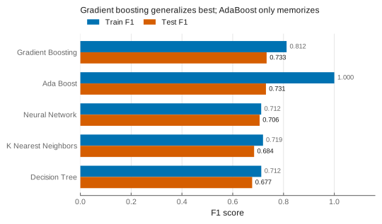
| ML Model | Train F1 | Test F1 |
|---|---|---|
| Decision Tree | 0.712 | 0.677 |
| Gradient Boosting | 0.812 | 0.733 |
| Neural Network | 0.712 | 0.706 |
| Ada Boost | 1.000 | 0.731 |
| K Nearest Neighbors | 0.719 | 0.684 |
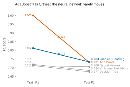
Gradient boosting was selected as the final model. Two things in the table are worth reading carefully. AdaBoost’s perfect training F1 buys it almost nothing on test (0.731 against gradient boosting’s 0.733), which is a large train/test gap rather than a failure to generalize: the gap diagnoses how the model fits, not how well it predicts. And the neural network has the narrowest gap of any model tried while scoring below the ensembles, which is worth noticing without treating a small gap as a selection criterion when held-out scores are available.
Reading the same table as a question about generalization rather than raw score makes the difference visible:
Deployment
The final model was serialized and deployed inside a web application built with Plotly and Dash, hosted on Render. A user selects two players and a match context; the application returns the predicted winner alongside the historical statistics that drove the prediction, so the number is never presented without the evidence behind it. Feature datasets were exported to CSV so the application runs without the original PostgreSQL database.
Report
- Tennis Match Predictions Project Report: full methodology, dataset selection trials, feature engineering, and the learning and validation curves for the final model.